Cellular Automata - from Game of Life to Compound

Some time ago, thanks to Softology and slackermanz with his awesome shaders, I got addicted to the Multiple Neighborhoods Cellular Automata. That was very fun, and exploring it let to multiple awesome rules and pictures, but then at some point I decided to add an extra complication to it.

And this is where those pictures come from.

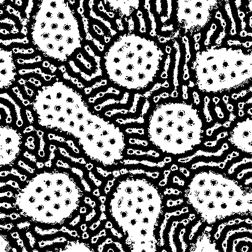
So let’s take a look at the evolution, from Game of Life to the Compound weirdness. All provided code is in Processing (Java mode).

So, what is a Cellular Automaton?

A Cellular Automaton (CA) consists of a grid of cells (commonly square, but can be hexagonal or anything weird). It is not a must, but here we will stick to 2d grids. Each cell can be in one of a finite number of states. Here, we will work with binary states - 0 or 1, on or off, but it does not have to be. In fact, you can create multistate automata with similar behaviour. An initional state (generation t = 0), is selected by assigning a set to each state either at random or following some pattern of our choice.

Then, for each cell, we define a neighborhood relative to it. For example, we could take the cell imediateli above and below a cell.

We obtain the next generation (generation t = t + 1) by applying a fixed rule to all cells (simultaneously, in all our examples). The rule is some mathematical function, or a set of functions that determines the new state of a cell based on its current state and the states of cells in the neighborhod.

Game of Life

There are many great explanations and implementations of Game of Life, so I won’t provide too many details here.

We have a square grid and 2 states (alive and dead). The neighborhood of a cell consists of 8 cells that are horizontally, vertically, or diagonally adjacent to it.

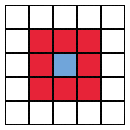
The rules are simple:

• a live cell with 2 or 3 live neighbors lives on
• a live cell with fewer than 2 or more than 3 live neighbors dies
• a dead cell with 3 live neighbors becomes alive
• else, it remains dead

So, how does it work?

We will work with a n x n square grid, where each pixel corresponds to a cell. Same height and width are not a must, but they sure help to simplify the notation. You start with two 2D arrays - lets call them A and B. A contains the current states os all cells, while B will store the state at t+1.

We populate A with random 1’s and 0’s. In the example below, I used a probability of 10% for 1, but when exploring more complex patterns, I recommend either using perlin noise or a gradient, to ensure that patterns that require a high density seed will still develop and you will not miss them.

Then, we iterate through A. For each cell (x,y), we calculate the sum of the 8 neighbor cells. Based on this sum (and in this case the state of the cell itself), we apply the rules described above. The result is stored in B.

Finally, update A with values from B, and plot the new generation on screen.

Download Processing code here

As you may have noticed, there is a small issue with the cells such as (0,0): part of the neighborhood is outside of our defined grid. There are several ways to approach this problem:

1. Skip those cells, as I did above. The benefit is that its easy, stable and fast, but then you end up with some weirdness on borders and may not be viable with larger neighborhoods.
2. Wrap your grid into a torus: so, for example, the left neighbour of (0,0) will be (n-1, 0), and so on. This requires some extra effort and very likely some extra calculations. And, as consequence, a performance loss.
3. Instead of storing a grid, store the coordinates of the “alive” cells. This may be somewhat disastrous for expanding automata.

Larger than Life

Larger than Life is a generalization of Game of Life, described by Kellie Michele Evans in 1996. The basic idea is that, instead of using a 3 x 3 neighborhood, we can use a (2r + 1) x (2r + 1) neighborhood, where r is some positive integer. For example, below a neighborhood for range r = 3:

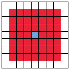
Then, the rule is changed to:

• If a cell is dead, it will become alive if s, the number of living cells in the neighborhood, is in the closed interval $[b_1, b_2]$.
• If a cell is alive, it will remain alive only if s is in the closed interval $[a_1, a_2]$.
• Else, the cell either remains dead or dies.

The implementation is pretty much identical to Game of Life.

Download Processing code here

Different Neighborhood Shapes

Now, following Slackermanz and his code here we can make another step further from Game of Life and into the weird land. We already started working with arbitrarely large neighborhoods, so lets also use some different shapes for them.

For example, a neighborhood like this:

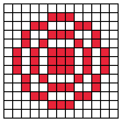
We will also simplify our rules a bit:

• If s, the number of living neighbours of a cell, satisfies $a \leq s \leq b$, the cell becomes alive if it was dead, and remains alive if it was alive.
• If s, the number of living neighbours of a cell, satisfies $c \leq s \leq d$, the cell dies if it was alive, and remains dead otherwise.
• Else, the cell state remains unchanged.

To see how this works, check out the link below. Observe that, since our neighborhood is now pretty irregular, instead of using a loop I just list all the cells that belong to it instead.

Download Processing code here

Overall, while this is pretty flexible, not all neighborhoods produce equally interesting results. In general, I found that neighborhoods that are less dense are more prone to producing degenerate or excessively chaotic patterns. On the other hand, denser neighborhoods demand more computations. While this is irrelevant for small neighborhoods, when working with ones with range $r > 100$, it becomes a bigger deal, and may require some careful tweaking and experimenting.

In short, if you keep getting crappy patterns only, you may need to check the neighborhoods, and maybe add a couple of extra points to them.

Multiple Interval Rules

Next step is to make the rule a bit more complicated. So far, we used a single interval for each rule, and it was fine, but using a union of disjoint intervals may be fun too, and add some extra textures to it.

Lets update the rule for multiple intervals:

• If the number of living neighbours of a cell is contained in $\bigcup_i (a_i \leq s \leq b_i)$, the cell becomes alive if it was dead, and remains alive if it was alive.
• If the number of living neighbours of a cell is contained in $\bigcup_j (c_j \leq s \leq d_j)$, the cell dies if it was alive, and remains dead otherwise.
• Else, the cell state remains unchanged.

Download Processing code here

Notice that you not necessarely should follow the interval order. While of course its nice and easy to setup first all the “alive” intervals, and then all the “dead” intervals, as you tweak it, things may mess up, because you will want to try things such as “what if, instead of having the cells live here, I make them die”, and then tweak the parameters to obtain overlapping intervals.

Multiple Neighborhood Automata

The part that brings the most of the spice to Slackermanz’ automata is the use of multiple neighborhoods.

So instead of working with one neighborhood as before, we have m of them. With $N_k$ being the k-th neighborhood, the rule now looks like this:

• For $k = 1, ..., m$
  • If sum of cells over neighborhood $N_k$, $\sum_{N_k} (cells) \in \bigcup_i (a_{k,i} \leq s \leq b_{k,i})$, the cell becomes alive if it was dead, and remains alive if it was alive.
  • If $\sum_{N_k} (cells) \in \bigcup_j (c_{k,j} \leq s \leq d_{k,j})$, the cell dies if it was alive, and remains dead otherwise.
  • Else, the cell state remains unchanged.

Download Processing code here

Notice that the order of the neighborhoods in the rule will have an effect on the final result. In short, the first neighborhood has usually the least effect, and the last one, the most.

As you probably noticed at this point, the size of the features of the CA depends on the neighborhood range. For example, on the picture below, we have a Multiple Neighborhood Cellular Automaton with three neighborhoods. First one, with $r = 6$, is responsible for the texturing. The second one, with $r = 14$ produces the worm-like structures. Finally, the third one, with $r = 50$ is responsible fro the larger structures.

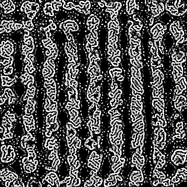
Following this logic, it is a good choice to order your neighborhoods by range, and apply rules to the smaller ones first. If done the other way around, the effect of the small neighborhoods may reduce or even remove entirely the effect of the large ones.

Compound Rules

After playing extensively with the ideas above, I started to think about the possibilities to complicate the rules even further. And this is how the idea of using several rules together as a function of a neighborhood was born.

We define several Multiple Neighborhood rules, and then apply one of them based on the sum of cells over another neighborhood. The basic rule structure, given a neighborhood $N_0$, is:

• If sum of cells over neighborhood $N_0$, $\sum_{N_0} (cells) \in \bigcup_i (a_{0} \leq s \leq b_{0})$, the we apply our first Multiple Neighborhood rule:
  • For $k = 1, ..., m_1$
    • If sum of cells over neighborhood $N_{1,k}$, $\sum_{N_{1,k}} (cells) \in \bigcup_i (a_{1,k,i} \leq s \leq b_{1,k,i})$, the cell becomes alive if it was dead, and remains alive if it was alive.
    • If $\sum_{N_{1,k}} (cells) \in \bigcup_j (c_{1,k,j} \leq s \leq d_{1,k,j})$, the cell dies if it was alive, and remains dead otherwise.
    • Else, the cell state remains unchanged.
• If sum of cells over neighborhood $N_0$, $\sum_{N_0} (cells) \in \bigcup_i (c_{0} \leq s \leq d_{0})$, the we apply our first Multiple Neighborhood rule:
  • For $k = 1, ..., m_2$
    • If sum of cells over neighborhood $N_{2,k}$, $\sum_{N_{2,k}} (cells) \in \bigcup_i (a_{2,k,i} \leq s \leq b_{1,k,i})$, the cell becomes alive if it was dead, and remains alive if it was alive.
    • If $\sum_{N_{2,k}} (cells) \in \bigcup_j (c_{2,k,j} \leq s \leq d_{2,k,j})$, the cell dies if it was alive, and remains dead otherwise.
    • Else, the cell state remains unchanged.
• Else, the cell state remains unchanged.

Of course, you can use more than one compound rule, and make it as complicated as you want. You can compound on compound and so on.

Just in case all that stuff above looks complicated, lets go through my own code. Download Processing code here

First of all, this was the stage when I switched to .glsl shaders entirely. Default processing is just too slow for those things, specially with large neighborhoods. So now, the processing code is only used to feed the rule parameters into shader, and then plot the results on screen. The actual rules are contained in the .glsl file in the data folder.

In this specific example, I use 4 neighborhoods:

• $N_0$ with range $r = 100$, the large neighborhood that produces the main shapes
• $N_1$ with range $r = 4$, the small texture neighborhood common for both rules
• $N_{2,1}$ and $N_{2,2}$, both with range $r = 14$

The rule $R_0$ is based on the largest neighborhood, and is the “condition” rule to chose between the other two:

• If $\sum_{N_0} (cells)$ is lower or equal to some $b_0$ value, then apply rule $R_1$
• If $\sum_{N_0} (cells)$ is greater or equal to some $c_0$ value, $c_0 \geq b_0$ then apply rule $R_2$

Then, rule $R_1$ is a Multiple Neighborhood and Multiple Interval rule, based on neighborhoods $N_1$ and $N_{2,1}$. Meanwhile, rule $R_2$ is based on neighborhoods $N_1$ and $N_{2,2}$. You can find more details on those rules in the provided code - the overall idea is very similar to the Multiple Neighborhood example provided in previous section.

Outputs of this rule, first one for the parameters provided in the example, and other for a diferent parameter set.

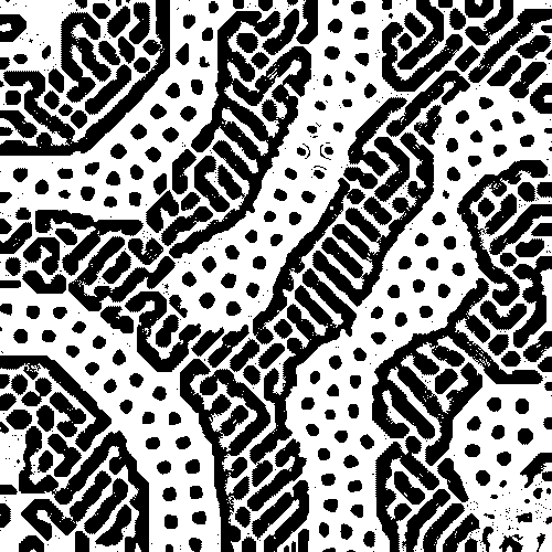
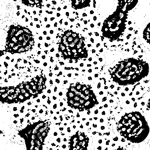
After playing a bit, you will notice that this is where sheer experimentation becomes very inefficient, due to the interaction between two different rules, and the number of parameters you can tweak.

The first thing you can do to improve this is to separate the rules. A good workflow is to first find a parmset that produces nice results for $R_1$ - you can either tweak $R_0$ so that $R_1$ is applied always (set some insanely high $b_0$), or even do it in a separate CA, using $R_1$ as the only rule. Then, you do the same for $R_2$ (use $c_0 = 0$, or build a CA with just $R_2$). Then, you can fix the parameters for $R_1$ and $R_2$, and only tweak the parameters $b_0$ and $c_0$ for $R_0$ until you get some stable outcome.

You will quickly gain some more intuition on how to combine rules more efficiently. For example, a $R_1$ or $R_2$ with very unstable output will likely produce an equally chaotic result for the whole system. In some cases, the other rule may help to stabilize it, but in general using rules that lead to quickly changing results may not be such a good idea.

In the setup i shared, specifically, a good combination of rules is one where $R_1$ leads to a higher density of alive cells than $R_2$. Actually, you will soon notice that this example is actually bad, in a sense that, as the rules are defined, $R_2$ tends to produce higher density outputs, and a more flexible and rich ruleset would be the one where $R_1$ and $R_2$ are switched.

Experiment and have fun =)