Word2Vec and Game of Thrones - Part 2

Following this post by Phelipe Teles, and because it takes so long until the episode 3, I decided to play a bit with Game of Thrones subtitles. And since I wanted to use Word2Vec for a while, it was an obvious choice.

Word embedding is a very popular way to represent vocabulary. It can capture context, semantic and syntactic similarities and so on. In short, an embedding is a vector representation of a certain word, and Word2Vec, developed by Tomas Mikolov, is a method to construct such embeddings.

Now, we should not expect too much from this. Word2Vec hates small datasets. And Game of Thrones subtitles are a small dataset, with only 40k observations. Even worse, the subtitles usually consist of very short sentences, in fact most of them with 5 words or less, so we are not getting much context here. Very likely, our model will lead to some weird and inconsistent results.

Word2Vec training

Now we can fit a Word2Vec model from gensim to our data.

Lets take a look at the parameters. All words with counts lower than min_count will be ignored.

Then, window is the maximum distance between the current and predicted word within a sentence. As described in Dependency-Based Word Embeddings, larger windows will capture more of the topic information, while smaller windows capture more of the semantic function of the word. Since we deal mostly with very short (if not one-word) sentences, anything above 3 makes no huge difference.

There is no point in using a large size here: we have a small dataset, so doing it would only lead to chaos and longer training time.

Finally, as reported by Mikolov, the Skip Gram works better for small datasets, so we will use sg = 1.

from gensim.models import Word2Vec

#set up the model
Word2Vec_model = Word2Vec(min_count=10, window=3, size=10, sg = 1)

#build vocabulary
Word2Vec_model.build_vocab(s_lemm)

#train
Word2Vec_model.train(s_lemm, epochs=20, 
                     total_examples=Word2Vec_model.corpus_count) #num of sentences

One that does not match

We got our Word2Vec model nice and trained, but does it make sense? We can look at some basic similarities to check that out, so prepare for some nonsence. Also, keep in mind that, due to the size of the dataset, the results of different runs will not necessarely converge to the same thing.

Word2Vec has several built in functions for this, and we will start with .wv.doesnt_match. The input of this function is a list of words, and the output is the word that doesn’t go with the others. Can it identify the bastard among the Stark children?

Word2Vec_model.wv.doesnt_match(['sansa', 'arya', 'jon', 'rickon', 'bran', 'robb'])

The answer is “jon” and it got it right.

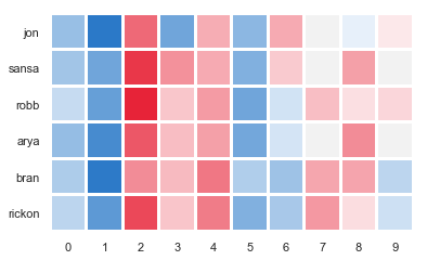
We can look more in depth into how this was done, by extracting the embeddings corresponding to each of the names and plotting the values in a heatmap. For plotting, we will use seaborn.

The first step is to get the positions of words of our interest. Then, we extract the corresponding embeddings - just call .wv.vectors_norm (I organized everything into a DataFrame to make it look pretty). This DataFrame can now be plotted with heatmap from seaborn.

import seaborn as sns
import matplotlib.pyplot as plt
sns.set(style="white")

def draw_factors_heatmap(words):
    #get words
    topwords = np.array(Word2Vec_model.wv.index2entity)
    #get the ids of words we are interested in
    ind = np.where(np.isin(topwords, words))[0]
    #extract values from word2vec
    data = pd.DataFrame(Word2Vec_model.wv.vectors_norm[ind, :], 
	                    index = topwords[ind],
                        columns = list(range(10)))
    #draw heatmap
    sns.heatmap(data, 
	            cmap = sns.diverging_palette(250, 10, s = 90, as_cmap = True),
                vmax = data.values.max(), vmin = data.values.min(), 
                square = True, linewidths = 2, cbar = False)
    plt.yticks(rotation = 0)
    plt.show()

#plot it
draw_factors_heatmap(['jon', 'sansa', 'arya', 'rickon', 'bran', 'robb'])

We can actually see what factors contribute the most for Jon being set as different from the rest of the pack.

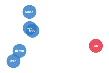
Another visualization option is to use PCA to map the embeddings to 2d. So we will import PCA from sklearn and, for some subset of words, create and fit a PCA model with 2 components. Of course, we could do it to all the embeddings first, and then extract the subset, but the spatial distribution in this case would be much worse.

Notice that the code below is for the unprettified version of the plot.

from sklearn.decomposition import PCA

def draw_pca(words):
    #get words
    topwords = np.array(Word2Vec_model.wv.index2entity)
    #get the ids of words we are interested in
    ind = np.where(np.isin(topwords, words))[0]
    #extract values from word2vec
    data = pd.DataFrame(Word2Vec_model.wv.vectors_norm[ind, :], 
	                    index = topwords[ind], 
                        columns = list(range(10)))
    #fit PCA with 2 components
    pca = PCA(n_components = 2)
    pc = pca.fit_transform(data)
    #plot
    plot = sns.regplot(pc[:, 0], pc[:, 1], fit_reg = False, marker = "o",
                       color = "white")
    #write text
    for i in range(len(ind)):
        plot.text(pc[i, 0], pc[i, 1], topwords[ind][i], 
	              horizontalalignment = 'center', 
                  verticalalignment = 'center', 
                  size = 'medium', weight = 'semibold')
    plt.show()

#plot
draw_pca(['jon', 'sansa', 'arya', 'rickon', 'bran', 'robb'])

The result makes a lot of sense. In the series, Bran and Rickon stay north, while Robb, Arya and Sansa go south, and Jon is a bastard and has a whole story of his own too.

Most similar

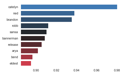
Then, we can also look for similarities, using .wv.most_similar. For example, let’s take a look at the words that are closest to ‘eddard’:

Word2Vec_model.wv.most_similar(positive = 'eddard', topn = 10)

The results make sense to a point. Catelyn is Eddard Stark’s wife, while Ned is his nickname. Brandon, Robb, Arya and Sansa are family.

def plot_bars(word, n):
    #get the most similar words
    data = pd.DataFrame(Word2Vec_model.wv.most_similar(positive=[word], topn = n))
    #plot
    ax = sns.barplot(x = 1, y = 0, data = data, 
            palette = sns.diverging_palette(250, 10, s = 90, n = n, center="dark"))
    #set labels
    ax.set(xlabel = '', ylabel = '')
    #set limits
    ax.set_xlim(min(data[1]) - 0.01, max(data[1]))
    plt.show()

#plot
plot_bars('eddard', 10)

But the results not necessarely may make much sense to humans. For example, the top 10 words closest to “Cersei” are:

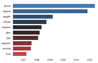
Also, “also” means we could maybe removed more stopwords here =)

Dendrogram

We can also try clustering the embeddings. Lets import linkage (for hierarchical clustering) and dendrogram (to visualize the results) from scipy.

from scipy.cluster.hierarchy import dendrogram, linkage

#distance matrix
dist = np.dot(Word2Vec_model.wv.vectors_norm, Word2Vec_model.wv.vectors_norm.T)

#clusters
h = linkage(dist, method='ward')

#dendrogram
P = dendrogram(h,  
            labels = np.array(Word2Vec_model.wv.index2entity),
            distance_sort = 'descending')
plt.show()

Since we are plotting the whole vocabulary, the results are pretty chaotic, but still capture some interesting relations. For example, we can see how kingsguard’s duty is to serve the king, and they swear an oath to protect him.

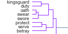
There are several other fun clusters, such as one with “valyrian”, “steel”, and “knife”.